The Transformer 1

Transformers have transformed (pun intended) all domains of machine learning – computer vision, natural language processing, or speech processing. The original paper is old by ML standards but the general idea of having an encoder/decoder architecture with an attention is still unsurpassed. At some point in my career, I felt that implementing a transformer from scratch would be very useful so grabbed the paper, opened my favorite editor of choice Visual Studio Code, and started coding. To prove that it works, I applied it to the task of mapping words to part-of-speech tags in Czech. I needed a sequence-to-sequence task and I having a dataloading code ready for this one made it an obvious choice.

This post is a detail of my journey of what I learnt and more importantly what I thought I knew but didn’t. As such, it contains a transformer implementation in Pytorch from scratch, dataloading code, training loop, an inference algorithm, and training graphs and performance metrics to prove it works.

This post assumes the reader is at least somewhat proficient with Pytorch. It is the first of two posts and discusses the following topics.

Introduction
- RNNs
- RNN-based encoder/decoder
- Attention
Basic transformer layers
- Feed forward network
- Multihead attention
- Positional encoding
- Input layers

Keywords: RNN, encoder/decoder, Luong attention, teacher forcing, auto-regressive decoding

1 Introduction

Imagine we want to do a sequence-to-sequence (seq2seq) machine learning. The input and output are sequences of various lengths and for our model to work well, the network shall condition output on inputs and previous outputs. This is what a transformer was originally designed for. However, why does it work so well? Well, to answer that it is best to look at what came before – recurrent neural networks (RNN) based encoder/decoder models. I am not going to describe RNNs and encoder/decoder architecture in details but rather focus on characteristics that give them their limitations. This will let me show that a transformer is an obvious evolutionary step over RNNs. Like going from copying books by hand to Guttenberg’s print.

1.1 RNNs

An RNN cell is best thought of as simple neural network and not a basic computational unit, i.e. a perceptron, and its purpose is to process sequences. The core idea is to process the sequence one element at a time and feed back the cell hidden state at time $t$ as an additional input at time $t+1$ to capture sequence context. The actual implementation of RNNs differ but we can use the diagram below for as illustration. The left part is a condensed version for the whole sequence, $\bold{x}$ is the input sequence, $\bold{h}$ is the hidden state, and $\bold{y}$ is the output sequence. The right part (past ‘Unfold’) is an element-by-element processing. It is typical to use zeros as initial hidden state as illustrated by ‘0’ being first hidden state.

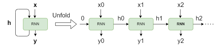
The core feature of RNNs is that as the cell processes the sequence element-by-element, the information gets accumulated in a hidden state vector $\bold{h}$ which is of a fixed size and the hidden state for the last element encodes the information from the whole sequence. RNNs have two main wekanesses:

Issue 1: the information capacity of the hidden state vector does not automatically scale with sequence length, running into a capacity issue for very long sequences
Issue 2: its sequential in nature and therefore slow (think of how GPUs love parallel processing)
Issue 3: models conditional probability of current output based on current input and all previous outputs: $P(y_i|x_i,y_1,...,y_{i-1})$

1.2 RNN-based Encoder/Decoder

A single RNN can be good to for simple seq2seq tasks but a better architecture later emerged – having one RNN to process input and one to produce an output. This idea is the core of RNN-based seq2seq models which contain two blocks, and encoder and decoder. This is a step up because it can now model conditional probability of current output based on all inputs and all previous outputs, solving Issue 3:

$P(y_i|x_1,...,x_n,y_1,...,y_{i-1})$

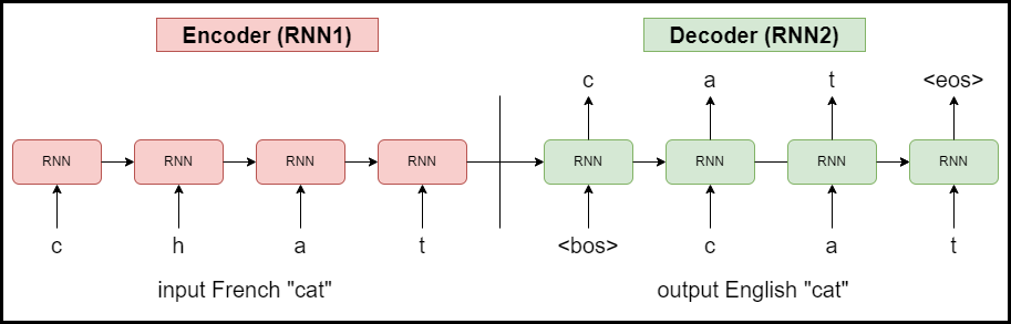
The model above is an illustration of basic RNN-based encoder/decoder model composed of two RNNs. The RNN1 processes the whole input sequence (word ‘cat’ in French) one letter at a time and encodes it into a fixed size hidden state vector. For the sake of simplicity, I omitted RNN1 outputs since we dont use them and also its initial hidden state $h_0$ . The final hidden state from RNN1 is then passed as an initial hidden state to RNN2, where it is used together with the a special beginning-of-sentence (<bos>) token to generate the first letter. The decoder then goes on to generate one letter at a time using the previous generated letters and hidden states. The process continues until the decoder generates a special end-of-sequence (<eos>) token, or a user-defined maximum number of tokens have been generated to avoid infinite loops. This method is also called an auto-regressive decoding. The training is done using a method called teacher forcing, when instead of using generated outputs, we use the true labels as RNN2 inputs. Such an architecture served its purpose but it has the same two main limitations:

Issue 1: the information capacity of the hidden state vector does not automatically scale with sequence length, running into a capacity issue for very long sequences
Issue 2: the process is still sequential and therefore slow

1.3 Attention

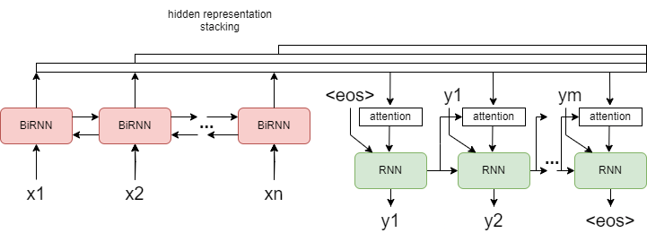
Attention was designed to solves both weaknesses: the bottleneck of hidden state vector, and the sequential processing. A possible implementation of a seq2seq with attention is illustrated in the diagram below. I still used RNNs, but only to illustrate the point.

The encoder is composed of BiRNNs to better represent left-right dependencies in the input and to generate a hidden representation (a vector) for each input element, stack these into a matrix, and feed them to the decoder. To illustrate encoder output stacking, notice that the number of bars over encoder is increasing, and ultimately the encoder is providing a representation for every input once it has processed the whole input sequence. Now, the decoder has a global access to all inputs through the attention block, which is illustrated by attention using decoder’s previous hidden state and all encoder outputs as inputs. The attention takes these and produces attention scores, a numerical representation of how current decoder input is dependent on all encoder outputs. This is fed into the RNN as additional input, a new output is generated, and the process continues as is typical for auto-regressive decoding. It is possible to carry over the encoder’s last hidden state as an initial hidden state for the decoder, but the transformers dont implement this so my illustration also lacks it. Just assume it is initialized with zeros.

2 Transformer architecture

The figure above is the architecture of The Transformer. The left part is the encoder, the right part is the decoder, and information flow between the two is through the Multi-Head Attention (MHA) layer. The encoder is a sequential stack of a Nx encoder layers, so is the decoder, and residual connections within blocks help with vanishing gradients and stabilize training. The main contribution of transformer lies in 1) replaces BiRNNs with self-attention to encode context inside encoder/decoder, 2) replaces hidden vector with cross-attention to facilitate information flow from encoder to decoder. For explanation, attention inside a module is called self-attention, attention between encoder/decoder is called cross-attention. Let us now explore their advantages over RNN-based seq2seq:

1) The decoder has a global access to all inputs a encoder output is a matrix that has as many rows as there are elements in the input sequences. We have solved Issue 1.
2) Doing all of this in parallel is thanks to how the attention block is designed, which we will discuss later. We have solved Issue 2.
3) Completely removes RNNs and their sequential nature and allows for parallel computations.
4) Attention has global overview of the whole sequence, unlike convolution (sees a small patch) or recursion (sees left-right).

Transformer architecture requires only implementing the following layers, because Add & Norm, linear, and softmax layers can be directly imported from Pytorch:

multi-head attention (MHA)
feed forward network (FFN)
positional encoding (PE)
input layer (I put embedding and PE layers into this)

The next step is to assemble them like a leggo. The provided code was optimized for readability not performance and can be run by importing a couple libraries. Finally, the following text assumes the transformer is used for an NLP task, so a sequence means a sentence and element means a word. I also use these terms interchangeably throughout the text.

The quadratic memory requirements of the attention matrix is an issue but we can solve that another day. The transformer uses a scaled dot-product attention (Luong attention) since it is easier to implement but harder to train but interested readers can also research Bahdanau attention.

2.1 Feed Forward network

The FFN is a sequence of a linear projection, ReLU, and a linear projection. Its task is to be a simple but powerful non-linear transformation of information as it flows through the model. This module is rather straightforward to implement, see the code below.

import torch
import torch.nn as nn
from typing import Callable, List, Optional, Tuple

class FFN(nn.Module):
    def __init__(self, input_dim: int, hidden_dim: int = 2048, device: str = "cpu"):
        super(FFN, self).__init__()
        self.fc1 = nn.Linear(input_dim, hidden_dim, device=device)
        self.relu = nn.ReLU()
        self.fc2 = nn.Linear(hidden_dim, input_dim, device=device)

    def forward(self, x: torch.Tensor) -> torch.Tensor:
        x = self.fc1(x)
        x = self.relu(x)
        x = self.fc2(x)
        return x

2.2 Scaled dot-product attention

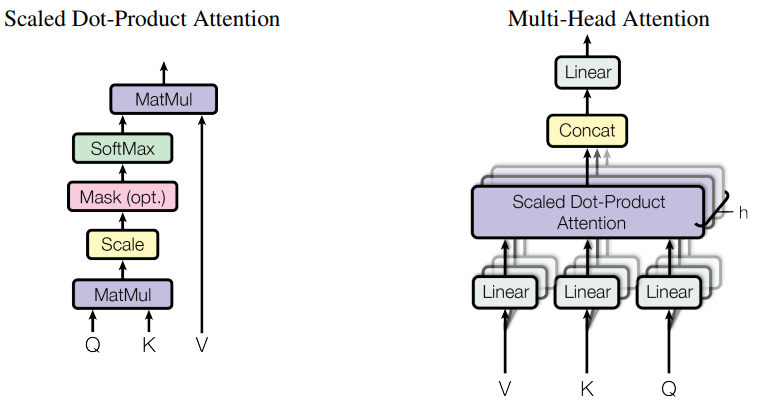
The MHA is by far the most complicated module. We will first implement a scaled dot-product attention (SDPA) (left image) and combine h-number of them into a single MHA (right image).

The fundamental concept of SDPA is query (Q), key (K), and value (V), which we can think of as distinct hidden representations every word produces for itself. The best analogy I can think of is that of searching on Google because these terms came from a retrieval systems anyway.. Query is akin to a search prompt submitted to Google engine. Key is the name of a website Google returns (or many website), and value is the URL address of the found website (or their respective URLs). In an NLP setting, Q, K, V are vectors which were obtained from word embeddings $X$ by applying trainable linear transformations without a bias or a non-linearity.

$Q = XW^Q, K = XW^K, V = XW^V$ ,

given that $W^Q, W^K \in \mathbb{R}^{d x d_k}$ and $W^V \in \mathbb{R}^{d x d_v}$ . Let us now explore the formula of SDPA to better understand its intent:

$Attention(Q,K,V) = softmax_j(\frac{QK^{T}}{\sqrt{d_k}})V$

$Q \in \mathbb{R}^{n x d_k}, K \in \mathbb{R}^{n x d_k}, V \in \mathbb{R}^{n x d_v}$ .

$QK^T$ represents how related Q and K are. Since Q and K are vectors, their product is a (n x n) matrix. $\frac{1}{\sqrt{d_k}}$ is the scaling, and softmax normalizes values for each $q_i$ across all $k_j$ to produce a probability density function (PDF). The result at this point is a rather neat matrix that shows how each word depends on other words. Finally, $(.)V$ produces the most relevant context representations as a PDF weighted average of value vectors. PSDA has one disadvantage and that is that easily overfits and requires tons of examples to train.

The code below implements ‘ScaledDotAttention’ layer by following the figure above. There are only a couple points I want to touch. Since our inputs are batched, we can make use of batch matrix multiplication (bmm) to do $QK^T$ and $(.)V$ . My code assumes the inputs are batches of shape (batch, time, features). `apply_Wo` is my own addition to see if I can improve results by applying one extra linear transform to attention output (also called context). `apply_mask` is a feature to restrict attention from looking into the future. The encoder self-attention sees the whole input but the decoder produces outputs one word at a time (remember auto-regressive decoding) which means it never sees future words. To simulate this behavior during training, for every word in our training sequence, we mask all future words so the self-attention has only access to past words. My implementation sets values in the upper triangular matrix to -Inf which results in softmax producing 0 probabilities for these. This is also called masked multi-head attention (MMHA)*. Class `AttentionProjection` encapsulates trainable linear transforms to produce Q, K, V vectors from attention inputs.

import torch
import torch.nn as nn
from typing import Callable, List, Optional, Tuple

class ScaledDotAttention(nn.Module):
    def __init__(
        self,
        model_dim: int,
        dk: int,
        dv: int,
        apply_Wo: bool = True,
        device: str = "cpu",
    ):
        super(ScaledDotAttention, self).__init__()

        self.input_projection = AttentionProjection(model_dim, dk, dv, device)
        self.dk = torch.tensor(dk, dtype=torch.float32, device=device)
        if apply_Wo:
            self.Wo = nn.Linear(dv, model_dim, device=device)
        else:
            self.Wo = nn.Identity()

        self.device = device

    def forward(
        self,
        query: torch.Tensor,
        keys: torch.Tensor,
        values: torch.Tensor,
        apply_mask: bool = False,
    ) -> torch.Tensor:
        B = keys.shape[0]
        
        q, k, v = input_projection(query, keys, values)
        scores = torch.bmm(query, keys.permute(0, 2, 1)) / torch.sqrt(self.dk)
        if apply_mask:
            T = query.shape[1]
            mask = torch.triu(
                torch.ones(B, T, T, dtype=torch.bool, device=self.device), 1
            )
            scores[mask] = float("-inf")
        
        weights = nn.functional.softmax(scores, -1)
        context = torch.bmm(weights, values)
        context = self.Wo(context)
        
        return context

class AttentionProjection(nn.Module):
    def __init__(self, model_dim: int, dk: int, dv: int, device: str = "cpu"):
        super(AttentionProjection, self).__init__()
        self.Wq = nn.Linear(model_dim, dk, False, device=device)
        self.Wk = nn.Linear(model_dim, dk, False, device=device)
        self.Wv = nn.Linear(model_dim, dv, False, device=device)

    def forward(
        self,
        q: torch.Tensor,
        k: torch.Tensor,
        v: torch.Tensor,
    ) -> Tuple[torch.Tensor, torch.Tensor, torch.Tensor]:
        return self.Wq(q), self.Wk(k), self.Wv(v)

2.3 Multi-head attention

Now, MHA is really a stack of SDPAs. The idea is to split one large SPDA into a stack of multiple smaller ones and merge the outputs back again (ResNet uses the same trick). The reason for using this trick to avoid large matrix multiplications and the propensity of attention to overfocus on a single word in the softmax. MHA forces the model to pay attention to more words at the same time. Its worth noticing that one large SPDA is identical to MHA, if the respective dimensionalities match. The code below is the implementation that makes use a `nn.ModuleList`.

import torch
import torch.nn as nn
from typing import Callable, List, Optional, Tuple

class MultiHeadAttention(nn.Module):
    def __init__(
        self, model_dim: int, dk: int, dv: int, heads: int, device: str = "cpu"
    ):
        super(MultiHeadAttention, self).__init__()
        assert dk % heads == 0
        assert dv % heads == 0

        self.att_list = nn.ModuleList(
            [
                ScaledDotAttention(
                    model_dim,
                    int(dk / heads),
                    int(dv / heads),
                    apply_Wo=False,
                    device=device,
                )
                for _ in range(heads)
            ]
        )
        self.Wo = nn.Linear(dv, model_dim, device=device)

    def forward(
        self,
        query: list[torch.Tensor],
        keys: list[torch.Tensor],
        values: list[torch.Tensor],
        apply_mask: bool = False,
    ) -> torch.Tensor:
        context = [
            att(q, k, v, apply_mask)
            for att, q, k, v in zip(self.att_list, query, keys, values)
        ]
        context = self.Wo(torch.cat(context, dim=-1))
        return context

*MMHA is also used to train so called causal (streaming) models, a model that can respond in real-time to the input instead of waiting for the whole sequence. To achieve this we need to restricts encoder’s access to the future the same way we do for the decoder.

2.4 Positional encoding

Position encoding (PE) task is to encode relative or absolute order of elements in a sequence. The paper argues that this is necessary because the model lacks recurrence or convolutions. Just think back to how the attention is calculated using Q, K, V – the process is completely agnostic to element order. Without it, a sequence “dog ate cat” and “cat ate dog” would seem identical, although we can understand that their meaning is reversed. It is possible to use a trainable matrix as PE, but the authors’ decided to use sines and cosines of different frequencies, defined by the following formulas:

$PE_{(pos,2i) = sin(pos / 10,000^{2i/d})}$

$PE_{(pos,2i+1) = cos(pos / 10,000^{2i/d})}$ .

$pos$ is the element’s position index in the sequence (word index in a sentence), $d$ is word embedding dimensionality, and $i$ is the embedding dimension. The authors hypothesize that using geometric functions would allow model to learn to attend to relative positions. Since PE and word embeddings have the same dimensionality, the two can be summed to create inputs to encoder/decoder layers.

PE is a matrix that contains the same values for all sequences, only its $pos$ dimensionality changes based on sequence length. Therefore, if we assume a maximum number of words if any sentence we can encounter, we can precompute the PE matrix for speed. The image below illustrates a PE of (64×256)-dim where the rows are word positions and column are embedding indexes. The sines and cosines occupy each 1/2 of the image (on why is that later) instead of being interleaved as the formula dictates.

The code below is the implementation with a couple design choices I made. 1) I chose to use a precomputed PE matrix controlled by the ‘max_seq_len’ parameter. This was an arbitrary number I knew was much bigger than any sequence length in my dataset. During a call, the module figures out the sequence length and takes only that many rows of the PE matrix. 2) I decided to concatenate sines and cosines instead of interleaving them since PE is followed by a fully connected layer which is agnostic to positions.

import torch
import torch.nn as nn
from typing import Callable, List, Optional, Tuple

class PositionEncoding(nn.Module):
    def __init__(self, max_seq_len: int, pe_dim: int, device: str = "cpu"):
        """
        Pre-computed for speed, figure out actual x_length during inference.

        max_seq_len: max number of words in a sequence
        pe_dim: position encoding dim which equals last dimension of input
        """
        super(PositionEncoding, self).__init__()
        self.max_seq_len = max_seq_len
        self.pe_dim = pe_dim

        assert pe_dim % 2 == 0

        d = int(pe_dim / 2)
        self.pe = torch.empty(max_seq_len, pe_dim, dtype=torch.float32, device=device)
        for k in range(max_seq_len):
            g = k / (10000 ** (2 * torch.arange(d) / pe_dim))
            self.pe[k, :d] = torch.sin(g)
            self.pe[k, d:] = torch.cos(g)

    def forward(self, x: torch.Tensor) -> torch.Tensor:
        """
        Expect `x` to be tensor of shape [T,F] or [B,T,F].
        """
        if x.dim() == 2:
            k_dim = 0
            i_dim = 1
        elif x.dim() == 3:
            k_dim = 1
            i_dim = 2

        assert x.shape[k_dim] <= self.max_seq_len
        assert x.shape[i_dim] == self.dim
        xk_dim = x.shape[k_dim]

        x = x + self.pe[:xk_dim, :]
        return x

2.5 Input layer

The final block is an input layer to encoder/decode that consists of a word embedding and positional encoding, see the code below. The embedding is a simple lookup table that transforms words represented as one-hot vectors into vectors of real values. The important part is that the embedding layer is trained. I have added an additional dropout for experimental purposes.

import torch
import torch.nn as nn
from typing import Callable, List, Optional, Tuple

class InputLayer(nn.Module):
    def __init__(
        self,
        input_dim: int,
        model_dim: int,
        max_seq_len: int,
        dropout_p: float = 0.2,
        device: str = "cpu",
    ):
        super(InputLayer, self).__init__()

        self.dropout = nn.Dropout(dropout_p)
        self.embedding = nn.Embedding(input_dim, model_dim, device=device)
        self.position_encoding = PositionEncoding(max_seq_len, model_dim, device)

    def forward(self, x: torch.Tensor) -> torch.Tensor:
        x = self.embedding(x)
        x = self.position_encoding(x)
        x = self.dropout(x)
        return x

We have described all layers to build our transformer. The following post will discuss the assembly, demonstrate training and inference, and present results for the task of mapping words to part-of-speech tags in Czech.